Lotka Volterra System Tracking with Kalman Filter
Abstract
This article investigates the Kalman filter and its sub-variant algorithms’ performance on a Lotka-Volterra System tracking. This article reviews the system model built by the Lotka-Volterra equation. The concept of Kalman Filter, Extended Kalman Filter and Unscented Kalman Filter is demonstrated, and their modified algorithms are presented. We compare the performance of these algorithms using MSE, RMSE, Tracking Results and Processing Time. We showed that under the same performance level in our system, the EKF offers a more stable and fast-tracking solution. However, UKE offers a slightly better RMSE performance.
Introduction
The Kalman Filter provides a reliable solution in system tracking for linear systems. It estimates the system states and make predictions about unknown variables with noised measurements. However, for non-linear systems, the Kalman filter does not perform well since the system cannot be expressed in linear matrix form. Other Kalman Filter based sub-variant algorithms are designed for these non-linear Gaussian problems, such as Linearized Kalman Filter, Extended Kalman Filter, and Unscented Kalman Filter. In this article, our goal will be to implement and compare these algorithms for the non-linear system.
Although both Extended Kalman Filter and Unscented Kalman Filter perform well on non-linear system tracking, there are still debates on which one to choose in practical applications. Depending on the system complexity and algorithm design, the complexity of UKF and EKF are different. In the following section, we have reviewed some practical applications of UKF and EKF. These studies provide a comparative analysis of different Kalman Filter based algorithms under different physical scenarios.
System Model
Non-linear System
We consider a system described as classical predator-prey population dynamic system. The system consists of two different participants in the system exhibiting a trade-off relationship. In this case, we name them: prey and predator. The cycle dynamics start from the increasing population of prey. Then, the abundance of prey would increase the population of the predator. When the predator population increases, the population of prey decreases. Then due to a lack of food sources, the population of predators decreases which results in an increase in the population of prey.
Their population are described in equations below \eqref{eq:syseq1}. \ref{syseq2}
$$ \begin{gather} dx_{1t} = x_{1t} [r_1 - a_{12}x_{2t}] \label{eq:syseq1} \\ dx_{2t} = x_{2t} [-r_2 - a_{21}x_{1t}] \label{syseq2} \end{gather} $$
In this mode, \( dx_{1t} \) and \( dx_{1t} \) are the population densities of prey and a predator at time t. The \(dx_{1t}\) and \(dx_{1t} \) are the change rate for the population densities, The \( dx_{1t} \) and \( dx_{1t} \) are the natural growth and death rate for the predator and prey, and \( dx_{1t}\) is the interaction parameter between different species.
We assume the growth rate and species interaction parameters are fixed in the system, and we take one step approximation of the above equation to the approximated next time step state of our system as shown in equation.
$$ \begin{gather} x_{1,t+1} = \Delta t \cdot dx_{1,t} + x_{1,t} + v_{1}\\ x_{2,t+1} = \Delta t \cdot dx_{2,t} + x_{2,t} + v_{2} \end{gather} $$
The \( \Delta t \) here is the time step. Here, process noise \(v_1\) and \(v_2\) as zero mean and variance \( \sigma_1 \) and \(\sigma_2\). Clearly, our system is not linear. Thus it can be represented in a matrix form for state transition. We rewrite the system in equation below.
$$ \begin{equation} \begin{bmatrix} x_{1,t+1}\\ x_{2,t+1} \end{bmatrix} = f(\begin{bmatrix} x_{1,t}\\ x_{2,t} \end{bmatrix}) + \begin{bmatrix} v_{1}\\ v_{2} \end{bmatrix} \end{equation} $$
As for the measurement, we assume that we are able to measure the \(x_{n,1}\) and \(x_{n,2}\) directly with a certain variance. In this case, the measurement is linear. Then the measurement function can be written in equation below. The \(u_1\) and \(u_2\) denote measurement noise.
$$ \begin{equation} \begin{bmatrix} y_{1,t}\\ y_{2,t} \end{bmatrix} = \begin{bmatrix} 1 & 0\\ 0 & 1 \end{bmatrix} \cdot \begin{bmatrix} x_{1,t}\\ x_{2,t} \end{bmatrix} + \begin{bmatrix} u_{1}\\ u_{2} \end{bmatrix} \end{equation} $$
Linearized Kalman Filter
Kalman Filter(KF) works well on linear discrete-time dynamic system tracking due to its capability to capture the physical relationship inside the dynamics system. The process equation models the unknown physical state transition behind the system. The measurement equation below describes the relationship between observation and the physical state of the system.
$$ \begin{gather} x(n+1) = F(n+1,n)x(n) + V_1(n)\\ y(n) = C(n)x(n) + v_2(n) \end{gather} $$ The innovation process in equation below is introduced at each time step to correct the system prediction direction by comparing the new measurement and predicted measurement and observed measurements.
$$ \begin{equation} \alpha(n) = y(n) - \hat{y}(n | {y}_{n-1}) \label{eq:KFinoovation} \end{equation} $$
In a typical Kalman Filter design, the state transition matrix is fixed before the system processing. In our implementation for the KF, we propose to use \(f\) from equation above to complete the state prediction. The linearized transition matrix is given by taking the derivative of the state equation. The corresponding transition matrix is given in equation below.
$$ \begin{gather} F_{kf} = \begin{bmatrix} 1+\Delta t (r_1-a_{12}x_{2,n-1}) & 0 \\ 0 & 1-\Delta t (r_2-a_{21}x_{1,n-1}) \end{bmatrix} \label{eq:Ftran} \end{gather} $$
Based on the introduction above, we can write modify the KF algorithm using linearized transition matrix. The sudo algorithm is demonstrated below
function [x_n,K_n] = KF (x_n1,K_n1,y_n,f,fdf,Q_n,C_n,R_n)
F_n = diag(fdf(x_n1));

K_nn1 = F_n*K_n1*F_n' + Q_n;
x_nn1 = f(x_n1);

G = K_nn1*C_n'/(C_n*K_nn1*C_n' + R_n);
alpha = y_n-C_n*x_nn1;
x_n = x_nn1 + G*alpha;
K_n = K_nn1 - G*C_n*K_nn1;
end
Extended Kalman Filter
Another option for system estimation is using the Extended Kalman Filter(EKF). The Extended Kalman Filter linearizes the process equation and measurement equation by using the Jacobian matrix if necessary. By differentiation to get the approximated transition matrix $F$ and measurement matrix $H$.
$$ \begin{gather} \tilde{F} = \frac{\partial f}{\partial x} \\ \tilde{H} = \frac{\partial h}{\partial x} \end{gather} $$
Given the process equation, the state transition matrix is given in equation. The measurement function is a linear function, so we do not need to use the Jacobian matrix for it.
$$ \begin{gather} F_{kf} = \begin{bmatrix} 1+\Delta t (r_1-a_{12}x_{2,t-1}) & -\Delta t x_{1,t-1} a_{12} \\ \Delta t a_{21} x_{2,t-1} & 1-\Delta t (r_2-a_{21}x_{1,t-1}) \end{bmatrix} \label{eq:EKFtran} \end{gather} $$
The algorithm for the EKF is given as in the algorithm below. Notice that the EKF algorithm is similar to the KF algorithm. The only difference between the EKF and LKF above is the transition matrix.
function [x_n, K_n] = EKF(x_n1, K_n1, y_n, f, fJf, Q_n, C_n, R_n)

F_n = fJf(x_n1);
K_nn1 = F_n*K_n1*F_n' + Q_n;
x_nn1 = f(x_n1);

G = K_nn1*C_n'/(C_n*K_nn1*C_n' + R_n);
alpha = y_n-C_n*x_nn1;
x_n = x_nn1 + G*alpha;
K_n = K_nn1 - G*C_n*K_nn1;

end
Unscented Kalman Filter
The unscented Kalman Filter(UKF) is another sub-variant of the Kalman filter algorithm. It relies on the UT transformation, which is a technique for estimating the statistics for a random variable undergoing a nonlinear transformation. The basic idea behind UT transformation is summarized in 3 steps.
- select the a (2L+1) different sampling points (sigma points) to represent original x’s statistics
- Transform these sampling through nonlinear process $f$
- Get y’s statistics through these transformed sampling points \end{enumerate} Remark: These sampling points are not random but have to follow certain rules so that they can capture the mean and variance of the x. These rules are given in equation .
$$ \begin{gather} \chi_0 = \bar{x} \label{eq:ut1}\\ \chi_i = \bar{x} + (\sqrt{(L+\lambda)P_x})i, i=1,…L \label{eq:ut2} \\ \chi_i = {x} - (\sqrt{(L+\lambda)P_x}){i=L}, i=L+1,…,2L \label{eq:ut3} \end{gather} $$
Then passing these sigma points to the nonlinear function to get $\mathcal{Y}$
$$ \begin{equation} \mathcal{Y}_i = f(\chi_i), i=0,…,2L \end{equation} $$
The mean and variance for \( x(t+1) \) are estimated through weighted mean and covariance from \( \mathcal{Y} \) given in equation \ref{eq:uty1} and \ref{eq:uty2}. The weights are given in equation \ref{eq:w1}, \ref{eq:w2} and \ref{eq:w3}.
$$ \begin{gather} \bar{y} = \sum_i^{2L} W_i^{m}\mathcal{Y}i \label{eq:uty1}\ P{t+1} = \sum_i^{2L} W_i^{c} (\mathcal{Y}_i - \bar{y})(\mathcal{Y}_i - \bar{y})^T \label{eq:uty2} \end{gather} $$
$$ \begin{gather} W_0^m = \frac{\lambda}{L+\lambda} \label{eq:w1} \ W_0^c = \frac{\lambda}{L+\lambda}+1-\alpha^2 + \beta \label{eq:w2} \ W_i^c = W_i^m = \frac{1}{2(L+\lambda)}, i =1,…,2L \label{eq:w3} \end{gather} $$
The \(\lambda = \alpha^2(L+k) - L\) is a scaling parameter. The dimensionality of x determines the L. The $\alpha$ determines the spread of the sigma points, and it is set to a small positive value. The $k=3-L$ is another scaling parameter. The $\beta$ is used for incorporating knowledge on the prior distribution of x into sigma point selection.
The UKF first samples $x(t-1)$ for sigma points. Then, it does UT transformation to estimate the predicted states $x_p(t)$ and $P_p(t)$, which will be adjusted based on the innovation. Based on the $x_p(t)$, the UKF samples again for sigma points(set 2) and take measurements from these sigma points. These measurements from sigma points(set 2) will be used for calculating the estimated observation(y). Next, UKF would calculate the predicted covariance between x and y and the cross variance of y. The final step would be to calculate the Kalman gain and update the system based on all the information from above; The detailed algorithm is as follows.
function [x_n,P_n]=UKF(f,x_n1,P,h,y_n,Q,R)
L=numel(x_n1);
alpha=1;
ki=3-L;
beta=2; % for gaussian
lambda=alpha^2*(L+ki)-L;
Wm=[lambda/(L+lambda) 1/(2*(lambda+L))*ones(1,2*L)];
Wc=Wm;
Wc(1)=lambda/(L+lambda)+(1-alpha^2+beta);

Y = repmat(x_n1, 1,L);
Xsigmaset = [x_n1 Y+sqrt(L+lambda)*chol(P)' Y-sqrt(L+lambda)*chol(P)'];

LL=2*L+1;
x_np=zeros(L,1);
Xsigmap=zeros(L,LL);
y_np=zeros(L,1);
y_xsigmap=zeros(L,LL);
for i=1:LL
    Xsigmap(:,i)=f(Xsigmaset(:,i));
    y_xsigmap(:,i)=h(Xsigmap(:,i));
    x_np=x_np+Wm(i)*Xsigmap(:,i);
    y_np=y_np+Wm(i)*y_xsigmap(:,i);
end

P_np=(Xsigmap-x_np(:,ones(1,LL)))*diag(Wc)*(Xsigmap-x_np(:,ones(1,LL)))'+Q;

Pyy=(y_xsigmap-y_np(:,ones(1,LL)))*diag(Wc)*(y_xsigmap-y_np(:,ones(1,LL)))'+R;
Pxy=(Xsigmap-x_np(:,ones(1,LL)))*diag(Wc)*(y_xsigmap-y_np(:,ones(1,LL)))';
K=Pxy/Pyy;
x_n=x_np+K*(y_n-y_np);
P_n=P_np-K*Pxy';
end
Simulation
Simulation Setting
The setting is summarized in table \ref{tab:SimSetting}. This setting has been used in \cite{chow2004fitting} and \cite{chow2007unscented}. The $\Delta t$ is chosen as 0.01 for the step size. We set the measurement noise variance to 40 and process noise variance to 1. Setting a measurement variance is to differentiate the performance of different algorithms.
The parameter setting for UKF is $\alpha = 1$, $\beta=2$, $k=3-L = 1$. $x_{1,0}$ 400 $x_{2,0}$ 100 $r_{1}$ 1 $r_{2}$ 1 $a_{12}$ 0.0025 $a_{21}$ 0.005
For performance benchmarking, we will be looking at the algorithm’s ensembled RMSE and processing time between different algorithms.
Tracking Simulation
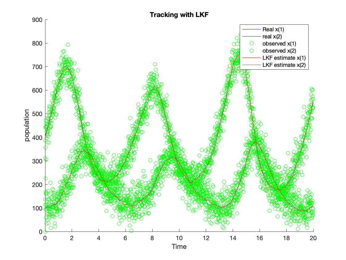
The figure in \ref{fig:tLKF} shows the tracking results using the LKF algorithm, and the figure in \ref{fig:tEKF} shows the tracking results using the EKF algorithm. The tracking results using the UKF algorithm are shown in \ref{fig:tUKF}. The green dots show the observation value. The red line is the estimation value from the algorithm. The blue line is the process value. The estimated values from LKF (red line) for $x(1)$ and $x(2)$ can follow the system process with some variance. Nevertheless, the variance is much lower compared with the observed variance. The estimated $x(1)$ and $x(2)$ from EKF can follow the system process with slight variance as well, and the estimated $x(1)$ and $x(2)$ from UKF can follow the system process as well. The EKF and UKF can outperform the LKF since their tracking noise is much lower than the LKF. We calculate their ensembled RMSE and accumulated processing time to compare these algorithms better to reveal their accuracy and complexity.


Performance Benchmarking
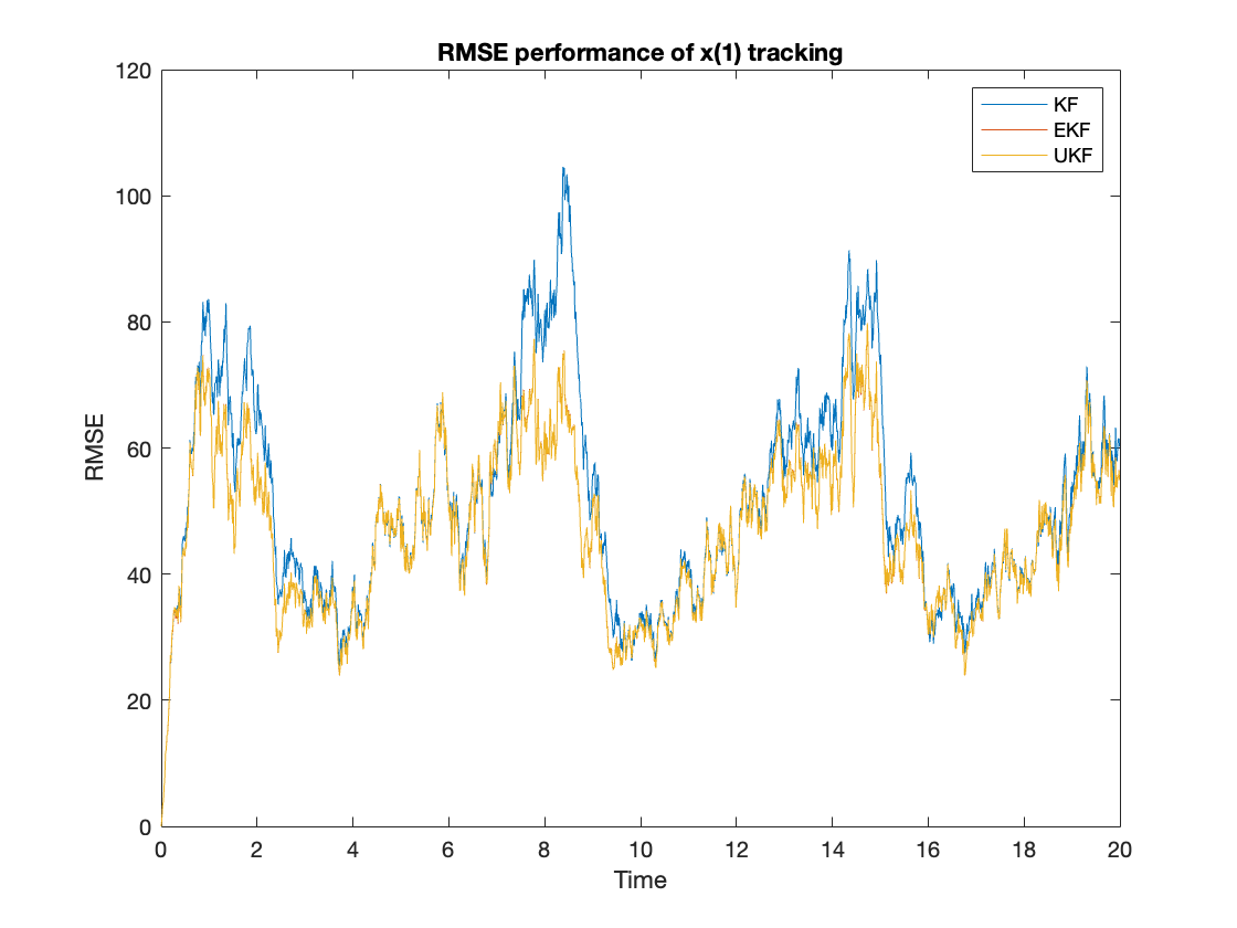
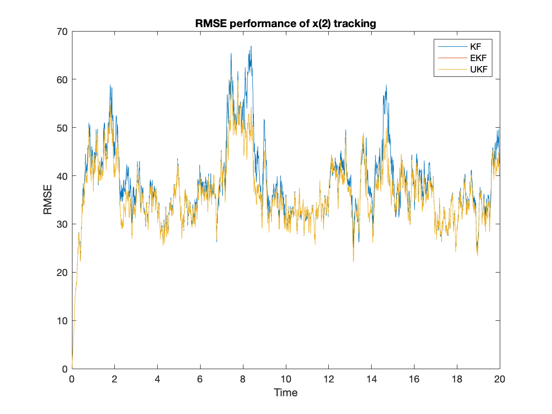
First, we compare the performance of different algorithms by calculating the ensembled RMSE of the tracking $x(i), i=1,2$ using equation \ref{eq:rmse}. The performance results are shown in figure \ref{fig:rmsex1} and \ref{fig:rmsex2}. The averaged RMSE is summarized at table \ref{tab:rmse}. From the figures, we can observe that the UKF and EKF clearly can outperform the KF. The UKF’s RMSE performance is slightly better than the EKF.
$$ \begin{equation} RMSE_{KF,EKF,UKF} = \sum_{n=1}^N |x(i) - x_{KF,EKF,UKF}(i)|^2 \label{eq:rmse} \end{equation} $$
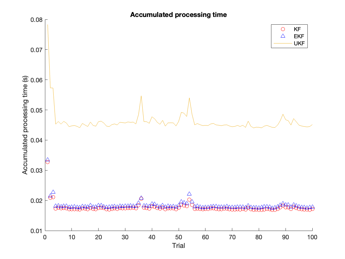
Next, we will be comparing the processing time of different tracking algorithms. We take 100 trails, and in each trial, we choose the tracking time as 2000 time slots. The processing time will be accumulated in each trail for each algorithm. The results are shown in figure \ref{fig:timecomp}. The averaged accumulated time is summarized in table \ref{tab:time}. We observe that the UKF is the most time-consuming among all these algorithms. The EKF and KF are close in terms of time performance, and EKF’s processing time is only slightly shorter than the KF’s processing time.
Conclusion
The above simulation shows that all three algorithms can track the Lotka-Volterra system with some variance. Among all three algorithms, UKF tracking lowers RMSE but has the highest computation cost. The processing time from UKF is much larger than the processing time from EKF and LKF. The RMSE from EKF is slightly larger than UKF, but its processing time is much lower than UKF. In such a case, the EKF is a better choice among all these candidate algorithms for the Lotka-Volterra system since it offers an outstanding accuracy with low complexity.
The main reason for the processing time difference is the operation complexity of different algorithms. For the EKF, the most time-consuming operation is the Jacobian matrix formulation. As for the UKF, the most time-consuming operation is the Cholesky factorization during sampling for the covariance matrix. Since the system’s order is only first order, the computation cost for Jacobian matrix formulation is low. Thus, in our case, the EKF’s complexity is lower than the UKF. Also, in most literature, the UKF can offer better performance in terms of RMSE than the EKF. Depending on the system, the performance gain from UKF can be really. For some cases, trading for high accuracy with high complexity is more desirable. In such conditions, the UKF is more desirable than EKF. Regarding stability, the UKF could fail during the iteration when performing Cholesky factorization. However, there are specific ways in literature to avoid this, such as iteratively factorization. However, this would downgrade the performance of UKF. Thus, in terms of stability, the EKF can outperform UKF.
The project can be extended to more complex system trackings with other non-linear filter algorithms for further work. For the Lotka-Volterra system, the tracking performance comparison is not that significant due to the complexity. To further benchmark, we can increase the system complexity. Also, there are other candidate algorithms for non-linear system tracking, such as the Particle filter. For further work, our goal is to implement other algorithms for comparison.
Code for System Tracking Evaluation
clear all;
close all;
clc;


delt = 0.01;
a12=0.0025;
a21=0.005;
v = 1;
u = 40;
Q_n = v^2*eye(2);
R = [u^2 0;0 u^2];

H_n=[1 0;0 1]; % Measurement Matrix
x(1:2,1) = [400; 100];

% EKF init
xekf(1:2,1) = x(1:2,1);
P(1:2,1:2,1) = eye(2);

% KF init
xkf(1:2,1) = [400; 100]; % Initial channel coefficients
Pkf(1:2,1:2,1) = eye(2); % Gaussian posterior covariance at time step 1


% UKF init
xukf(1:2,1) = [400; 100];
Pukf = eye(2);


f = @(x)[(1+delt*(1-x(2,1)*a21)) * x(1,1);(1-delt*(1-x(1,1)*a12)) * x(2,1)];
fdf = @(x)[1+delt*(1-x(2)*a21);1-delt*(1-x(1)*a12)];
fJf = @(x)[1+delt*(1-x(2)*a21) -delt*x(1)*a21;delt*x(2)*a12 1-delt*(1-x(1)*a12)];
h = @(x)[x(1);x(2)];

for n=2:2000
    % State propagation
    v_n = v*randn(2,1);
    x(1:2,n) = f(x(1:2,n-1)) + v_n;


    % Generate measurements
    w_n = u*randn(2,1);
    y_n = H_n*x(1:2,n) + w_n;

    %Linearized KF
    [xkf(1:2,n),Pkf(1:2,1:2,n)] = KF (xkf(1:2,n-1),Pkf(1:2,1:2,n-1),y_n, f,fdf,Q_n,H_n,R);

    %EKF
    [xekf(1:2,n),P(1:2,1:2,n)] = EKF(xekf(1:2,n-1),P(1:2,1:2,n-1),y_n, f,fJf,Q_n,H_n,R);

    %UKF
    [xukf(:,n), Pukf] = UKF(f,xukf(:,n-1),Pukf,h,y_n,Q_n,R);


end

t = [0:1999]'*delt;
figure
hold on
plot(t, x(1,:), 'b-');
plot(t, x(2,:), 'b-');

plot(t, xkf(1,:), 'r-');
plot(t, xkf(2,:), 'r-');
legend('Real x(1)','real x(2)','LKF estimate x(1)', 'LKF estimate x(2)');
xlabel('Time')
ylabel('population')
title('Tracking with LKF')
hold off

figure
hold on
plot(t, x(1,:), 'b-');
plot(t, x(2,:), 'b-');

plot(t, xekf(1,:), 'r-');
plot(t, xekf(2,:), 'r-');
legend('Real x(1)','real x(2)','EKF estimate x(1)', 'EKF estimate x(2)');
xlabel('Time')
ylabel('population')
title('Tracking with EKF')
hold off

figure
hold on
plot(t, x(1,:), 'b-');
plot(t, x(2,:), 'b-');

plot(t, xukf(1,:), 'r-');
plot(t, xukf(2,:), 'r-');
legend('Real x(1)','real x(2)','UKF estimate x(1)', 'UKF estimate x(2)');
xlabel('Time')
ylabel('population')
title('Tracking with UKF')
hold off
Code for Performance Evaluation
clear all;
close all;
clc;

%State space model


ensumbled_lc = zeros(6,2000);
processing_t = zeros(3,100);
for trial=1:100
d = zeros(6,2000);

delt = 0.01;
a12=0.0025;
a21=0.005;
v = 1;
u = 40;
Q_n = v^2*eye(2);
R = [u^2 0;0 u^2];

H_n=[1 0;0 1]; % Measurement Matrix
x(1:2,1) = [400; 100];
P(1:2,1:2,1) = eye(2);

% EKF init
xekf(1:2,1) = x(1:2,1);
P(1:2,1:2,1) = eye(2);

% KF init
xkf(1:2,1) = [400; 100]; % Initial channel coefficients
Pkf(1:2,1:2,1) = eye(2); % Gaussian posterior covariance at time step 1


% UKF init
xukf(1:2,1) = [400; 100];
Pukf = eye(2);

f = @(x)[(1+delt*(1-x(2,1)*a21)) * x(1,1);(1-delt*(1-x(1,1)*a12)) * x(2,1)];
fdf = @(x)[1+delt*(1-x(2)*a21);1-delt*(1-x(1)*a12)];
fJf = @(x)[1+delt*(1-x(2)*a21) -delt*x(1)*a21;delt*x(2)*a12 1-delt*(1-x(1)*a12)];
h = @(x)[x(1);x(2)];
    for n=2:2000
        v_n = v*randn(2,1);
        x(1:2,n) = f(x(1:2,n-1)) + v_n;


        w_n = u*randn(2,1);
        y_n = H_n*x(1:2,n) + w_n;

         %Linearized KF
        tic
        [xkf(1:2,n),Pkf(1:2,1:2,n)] = KF (xkf(1:2,n-1),Pkf(1:2,1:2,n-1),y_n, f,fdf,Q_n,H_n,R);
        processing_t(1,trial) = toc + processing_t(1,trial);
        d(1:2,n) = abs(x(1:2,n) - xkf(1:2,n));

        tic
        [xekf(1:2,n),P(1:2,1:2,n)] = EKF(xekf(1:2,n-1),P(1:2,1:2,n-1),y_n, f,fJf,Q_n,H_n,R);
        processing_t(2,trial) = toc + processing_t(2,trial);
        d(3:4,n) = abs(x(1:2,n) - xekf(1:2,n));


        % Compute for the ukf
        tic
        [xukf(:,n), Pukf] = UKF(f,xukf(:,n-1),Pukf,h,y_n,Q_n,R);
        processing_t(3,trial) = toc + processing_t(3,trial);
        d(5:6,n) = abs(x(1:2,n) - xukf(1:2,n));

    end
    ensumbled_lc = ensumbled_lc + d.^2;
end

ensumbled_lc = ensumbled_lc/100;
t = [0:1999]'*delt;
figure
plot(t, ensumbled_lc(1,:))
hold on, plot(t, ensumbled_lc(3,:))
plot(t, ensumbled_lc(5,:))
legend('KF','EKF','UKF')
xlabel('Time')
ylabel('RMSE')
title('RMSE performance of x(1) tracking')
hold off

figure
plot(t, ensumbled_lc(2,:))
hold on, plot(t, ensumbled_lc(4,:))
plot(t, ensumbled_lc(6,:))
legend('KF','EKF','UKF')
xlabel('Time')
ylabel('RMSE')
title('RMSE performance of x(2) tracking')
hold off

figure
hold on
plot(1:100, processing_t(1,1:100), 'ro');
plot(1:100, processing_t(2,1:100) , 'b^');
plot(1:100, processing_t(3,1:100)),'cd';
legend('KF','EKF','UKF')
title('processing time')